
Absolute Luminescence and Quantum Yield
Calibration, measurements & device insights: PLQY, QFLS, iVoc and PL mapping
Absolute photoluminescence and electroluminescence measurements quantify how efficiently semiconductor materials and devices emit light at different wavelengths. They also reveal the quantum yields of emission (PLQY, ELQY), the internal voltage of the excited electron–hole population (QFLS, iVoc). Combined with absolute PL mapping capability, these measurements give insight into recombination losses, stack efficiency potentials and spatial homogeneity of the semiconductor film or device.
Absolute Luminescence and Quantum Yield
When a semiconductor is excited, the resulting populations of electron and hole will annihilate one another in order to return toward equilibrium. This process is termed carrier recombination, and it can occur through radiative processes (luminescence), which emit photons, or through non-radiative processes, in which no photon is emitted. The balance between these pathways strongly influences the performance of optoelectronic materials and devices such as solar cells and LEDs.
A conventional PL measurement reports intensity in arbitrary units. Such a relative PL measurement is useful for comparing spectral shape, emission peak position and spectral shifts, but the signal cannot be directly interpreted as a number of emitted photons. An absolute PL measurement, by contrast, quantifies the emitted photon flux. It is reported in physical units (photons per second, or per second per unit area and energy interval) and provides quantitative information about both the spectral distribution and the total number of emitted photons.
Relative PL tells us where a material emits. Absolute PL tells us how much it emits.
Absolute electroluminescence (EL) measurements follow the same principle, except that the excitation is supplied by electrically injected charge carriers, delivered by a source-measure unit (SMU). The resulting EL spectrum provides information about the device under electrical injection (forward bias), i.e., with carriers supplied through its own contacts and transport layers. Comparing PL and EL can help distinguish (see Applications):
‣ Bulk recombination from injection or transport losses
‣ Material quality from contact limitations
‣ Changes in emission energy under applied bias
Quantifying the spectral distribution of a sample’s emitted photons in absolute terms makes it possible to determine luminescence quantum yields, quantify recombination losses, estimate the QFLS and iVOC, analyse intensity-dependent recombination and reconstruct pseudo-JV characteristics.
The distinction between relative and absolute PL is particularly important when comparing:
‣ Different materials or processing conditions
‣ Thin films and complete device stacks
‣ Different excitation intensities
‣ Different sample areas
‣ Different measurement geometries
‣ Samples with different emission spectra
Photon balance & quantum yield
The luminescence quantum yield (LuQY) describes the fraction of supplied excitation events that result in photons leaving the sample. In its most general form,
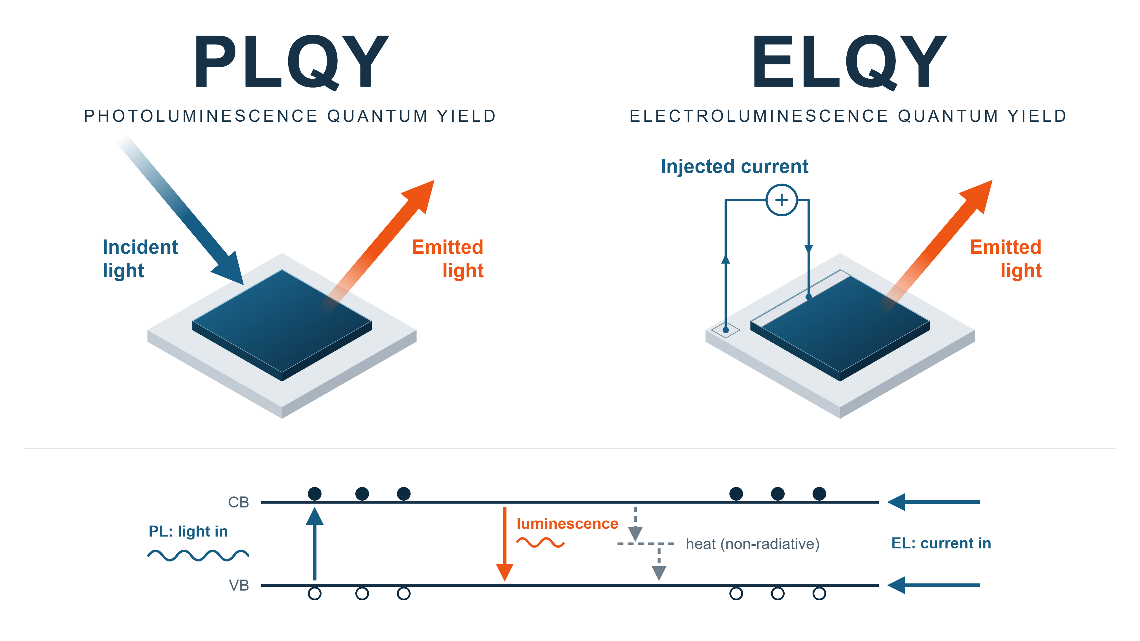
Under optical excitation, this quantity is referred to as the photoluminescence quantum yield (PLQY), while under electrical injection it is referred to as the electroluminescence quantum yield (ELQY).
For photoluminescence, PLQY is the ratio of the total emitted photon flux to the absorbed excitation photon flux:
Here, Φlum is the total emitted photoluminescence photon flux, Φexc is the incident excitation photon flux, and Φexc,R is the excitation photon flux that is reflected or otherwise remains unabsorbed. The denominator is therefore the absorbed excitation photon flux, not simply the light incident on the sample.
Integrating sphere and calibration
To distinguish the incident and reflected light from the sample's luminescence at the detector, an integrating sphere is used. An integrating sphere collects light emitted in all directions, homogenises it and measures the total optical output of a sample. This corrects for factors that influence the PLQY, such as the excitation intensity, reflected and transmitted excitation, re-excitation, sample structure, optical environment, photon escape and reabsorption.
In addition, a well-calibrated integrating-sphere system corrects for instrument-related factors, including:
‣ Wavelength-dependent optical losses
‣ Parasitic absorption in the sphere and sample holder
‣ Sample position and geometry
‣ Absorption of the sample by light scattered from the sphere wall
‣ Background and stray light
‣ Spectrometer sensitivity
This is particularly useful for thin films, textured samples, scattering materials and devices whose emission is not confined to a narrow collection angle. However, the sphere and spectrometer do not respond equally at every wavelength. The measurement system therefore requires a wavelength-dependent calibration of its optical throughput and detector response. This calibration converts the measured signal into an absolute spectral photon flux, which allows PL spectra to be compared quantitatively between different samples, excitation conditions and measurement sessions.
For all LuQY products, the equipment used for calibration is traceable to the national standards of EURAMET members (NPL, PTB, LNE, etc.), the US NIST or other national metrology institutes. Measurements that cannot be traced to national standards are traced to natural constants, other accepted standards or relational measurements. Calibrations are valid for one year.
Electrical injection and SMU
As mentioned earlier, when the sample emission comes from excitation events triggered by the charge carriers electrically injected from an SMU, the ELQY can be measured. For electrical injection with a sourced current ISMU, the number of elementary charges injected per second is
where q is the elementary charge. The electroluminescence quantum yield is therefore
Optical and electrical excitation can therefore be treated within the same photon-balance framework. A generalised expression describes PL, EL and combined optical and electrical excitation in a consistent photon-balance approach:
For a pure PL measurement, ISMU = 0. For a pure EL measurement, the optical excitation terms are absent. Operation in which the SMU sinks current, i.e. the device delivers photocurrent, is not covered by this LuQY definition.

With an integrated SMU, an electrical bias or current can be applied to the device while the optical system measures the resulting EL or PL. In addition to ELQY and absolute EL spectra, combining the SMU with calibrated optical detection gives access to:
‣ Bias-dependent absolute PL
‣ Current-dependent absolute PL
‣ Optical signatures of device degradation under electrical stress
‣ QFLS under applied bias or current
‣ Direct comparison of pseudo-JV and measured J–V characteristics
Both solar cells and LED applications benefit from resolving absolute PL as a function of electrical bias.
From calibrated spectra to photon flux
A spectrometer does not measure these total photon fluxes directly. Instead, it records a spectral photon flux density φ(E). The total photon flux is obtained by integrating the corresponding spectrum over photon energy:
PLQY can therefore also be written explicitly as
This formulation also shows why an absolute luminescence measurement is required. A conventional PL spectrum in arbitrary units can reveal the emission peak, linewidth and spectral shifts. In an absolute measurement, the recorded spectrum is calibrated to a physical spectral photon flux density, for example in photons s−1 eV−1. This, along with its integral, i.e., the total emitted photon flux Φlum, shows how many photons actually leave the sample and can be compared directly with the absorbed excitation.
The quantum yield is fundamentally a photon-number ratio, not a ratio of optical powers. It must therefore be calculated from spectra in photon-flux units rather than optical-power units. Photons at different wavelengths carry different energies, so integrating an optical-power spectrum would not give the correct photon-number ratio.
A higher PLQY generally indicates lower non-radiative recombination losses, provided samples are compared under equivalent excitation and optical conditions. Improved bulk material quality and better surface or interface passivation can therefore lead to a higher PLQY. However, PLQY should not be treated as a universal material constant: its value depends on the excitation level, sample structure and optical environment.
The measured PLQY is also an external quantum yield. It can differ from the internal quantum yield because photon escape (outcoupling), reabsorption and photon recycling determine how many internally generated photons ultimately leave the sample and are included in the measured luminescence flux.
While PLQY and ELQY describe how efficiently excitation is converted into emitted light, absolute luminescence contains additional information. Its absolute intensity is directly linked to the energetic state of the excited electron and hole populations. This link provides access to the quasi-Fermi-level splitting (QFLS).
Quasi-Fermi-Level Splitting
The quasi-Fermi-level splitting (QFLS) refers to the energy separation between the electron and hole quasi-Fermi levels under illumination or electrical injection.
In thermodynamic equilibrium, electrons and holes are described by a common Fermi level. Under illumination, excess electrons and holes accumulate in the conduction and valence bands, respectively, and the system is driven out of equilibrium. The electron and hole populations can then be described by separate quasi-Fermi levels, EFn and EFp.
The QFLS is defined as the energy difference between these quasi-Fermi levels and represents the electrochemical potential (free energy per electron–hole pair) of the non-equilibrium electron–hole population:

Dividing the QFLS by the elementary charge gives the implied open-circuit voltage, iVOC:
where q is the elementary charge.
The implied open-circuit voltage describes the internal voltage potential associated with the electron and hole populations in the absorber. In an ideal device with selective contacts and no additional voltage losses between the absorber and the external contacts, the open-circuit voltage VOC measured at the device terminals can approach iVOC.
In real devices and working samples, the QFLS and open-circuit voltage generally match with minimal error. However, the two can deviate from each other for a variety of reasons. This includes, for example, from non-ideal contacts and misaligned work functions, low mobility of absorber layers or interlayers, energy mismatch of transport layers, mobile ion & field-screening effects, or spatial variations of the quasi-Fermi levels. Assessing layer-by-layer difference between QFLS and VOC, measured under the same illumination, can therefore provide information about voltage losses that occur between the absorber and the external device contacts.
For more details, see Warby et al., Mismatch of Quasi–Fermi Level Splitting and Voc in Perovskite Solar Cells, Advanced Energy Materials 13 (2023), 2303135.
High-Energy Tail Fit
The QFLS can be extracted directly from the absolute luminescence spectrum using the High-Energy Tail (HET) fit. This approach is useful when the bandgap Eg and external quantum efficiency EQEPV of the sample are unknown. In case these quantities are defined, the LuQY calculates the QFLS from the PLQY with the approach from Unold et al. [1]
The HET method transforms the recorded absolute photon flux according to
Here, φlum(E) is the absolute PL/EL photon flux density, E is the photon energy, h is Planck's constant, c is the speed of light, a(E) is the absorptance of the sample, k is the Boltzmann constant, and T is the carrier temperature, commonly approximated by the sample temperature under thermalized steady-state conditions.
In this representation, the high-energy part of the luminescence spectrum becomes approximately linear. Extrapolating the fitted line to a transformed ordinate of zero gives the QFLS at its intersection with the photon-energy axis.
A shift in the spectral peak or onset may also indicate changes in, among other factors:
‣ Material composition
‣ Phase composition (e.g. phase segregation)
‣ Sub-gap or defect states
‣ Carrier density (e.g. band filling)
‣ Temperature
which can have direct impact on the PLQY and QFLS of the sample.
Stability testing for small and large area samples therefore finds benefit from analyzing stress-induced spectral shifts and associated changes in PL-derived metrics. (instrument options include LuQY Pro and LuQY Scanner.)
The HET method does not define a different type of QFLS. It is a method for extracting the same physical quasi-Fermi-level splitting from a suitable region of the absolute luminescence spectrum. The choice of fitting range is therefore important: a good linear fit alone is not sufficient if the selected spectral region does not satisfy the assumptions of the model.
Reading PLQY and QFLS Together
PLQY and QFLS depend on how many carriers are generated, because recombination mechanisms change with carrier density. Every non-radiative recombination pathways costs voltage to the device. Therefore, the PLQY and QFLS describe complementary aspects of the same excited semiconductor state. PLQY directly measures the fraction of radiative recombination pathways (i.e., it quantifies how efficiently absorbed excitation is converted into photons leaving the sample), while QFLS describes the energetic separation maintained between the electron and hole populations.
The connection between PLQY, QFLS and non-radiative voltage loss can be expressed as
relative to the corresponding radiative limit of VOC. This reference point describes the QFLS of the sample in the complete absence of non-radiative losses. In the absence of non-radiative losses, for example at the contacts or transport layers, every injected charge would reach the active layer and recombines there. In this case, the ELQY equals PLQY, assuming that the emitting species is always the same, and the excitation carrier density is the same.
PLQY tells you how close you are to that limit.
When samples are compared under equivalent excitation and optical conditions, stronger non-radiative recombination generally reduces the luminescence efficiency and the achievable QFLS. For instance, A PLQY of 1% means about 119 mV lost to non-radiative recombination at room temperature. Because the quasi-Fermi level splitting (QFLS) is the highest Voc a material can deliver, absolute PL lets you predict the voltage potential of films, half-stacks and full devices at every stage of fabrication. Improvements in bulk material quality, surface passivation or interface quality can therefore appear simultaneously as an increase in PLQY and an increase in QFLS.
At approximately room temperature, every order-of-magnitude reduction in PLQY corresponds to about 60 mV of additional non-radiative voltage loss:
| PLQY | Additional voltage loss |
|---|---|
| 100% | 0 mV |
| 10% | ≈ 60 mV |
| 1% | ≈ 120 mV |
| 0.1% | ≈ 180 mV |
PLQY tells us how efficiently the excited carrier population emits, while QFLS tells us how much internal voltage potential that population maintains. Evaluating both quantities together provides a more complete picture of non-radiative recombination losses and the performance potential of semiconductor materials and device stacks.
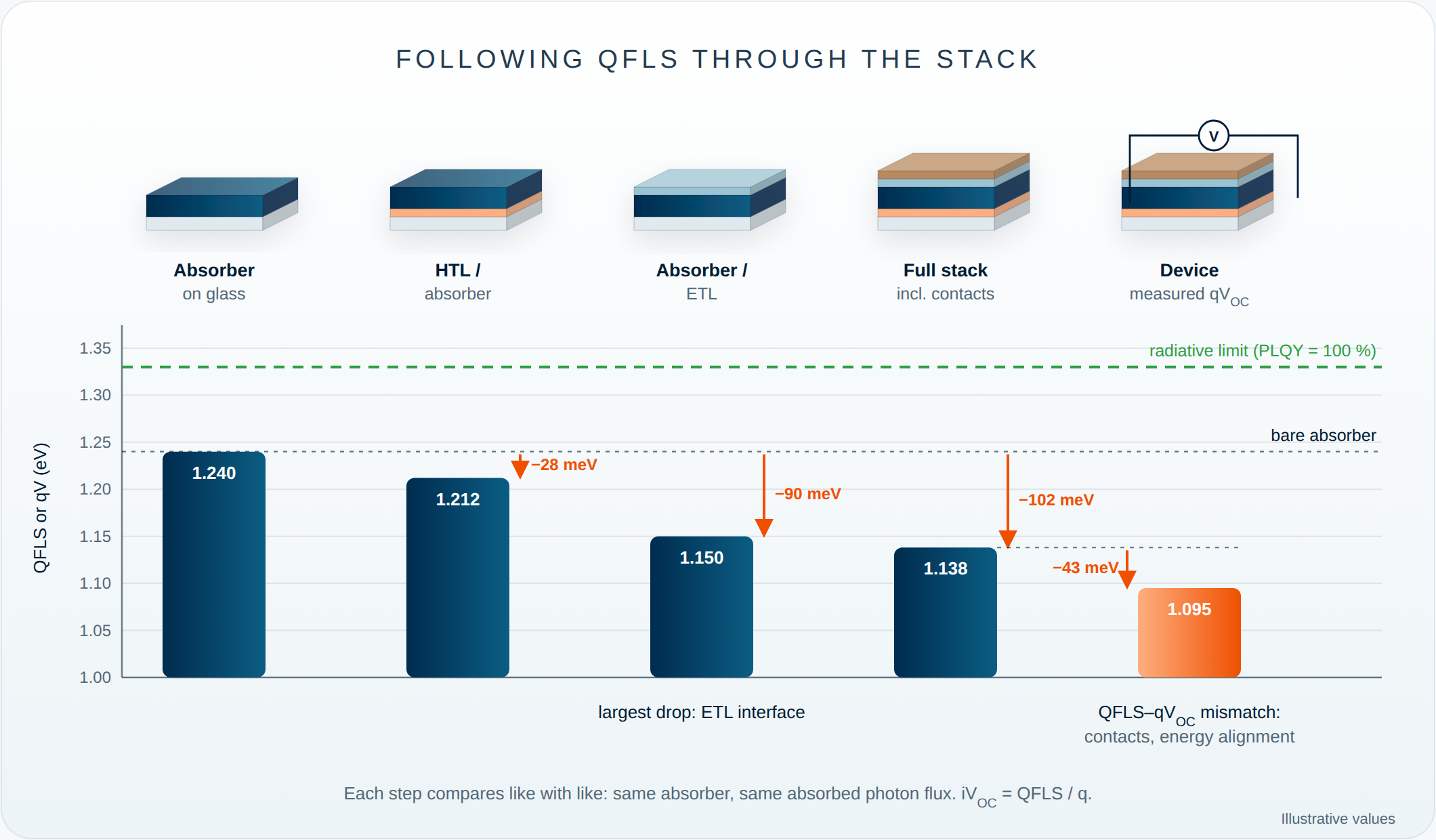
The ELQY provides an independent cross check for non-radiative losses of the device operated as an LED. Notably, for results to be relevant to solar-cell operation, the sample should be measured at a "1-sun equivalent" generation rate: the same number of carriers per second that the finished device would generate under AM1.5G sunlight.
Ideality Factor
The ideality factor describes how the quasi-Fermi-level splitting changes with excitation intensity.
When the excitation intensity is varied, the carrier density in the sample changes, and with it the quasi-Fermi-level splitting (QFLS). The slope of QFLS as a function of the logarithm of excitation intensity provides the ideality factor nid.
Here, G is the generation rate. For constant excitation spectrum and measurement geometry, Gis proportional to the excitation intensity. The dependence can therefore be evaluated directly from a QFLS versus excitation-intensity sweep.
When the excitation intensity is represented on a base-10 logarithmic scale,
At room temperature,
so that the slope of the QFLS dependence is approximately 59.5 nid meV per decade of excitation intensity.
In practice, the LuQY system records QFLS over a sweep of excitation intensities and determines the ideality factor from the measured trend. The ideality factor therefore provides a compact measure of how recombination changes with carrier density and operating conditions.
It can be used to compare materials and device stacks, evaluate changes in passivation or interfaces, and connect intensity-dependent luminescence measurements with device-relevant recombination behaviour. Its microscopic interpretation should, however, be treated with care: the ideality factor can depend on several recombination pathways, carrier statistics, energetic disorder and device structure, and should not be assigned to a single recombination mechanism without additional evidence.
Measuring QFLS over a range of excitation intensities provides not only the dominant recombination regime and the ideality factor, but also the basis for reconstructing an implied current-voltage characteristic.
Pseudo-JV curves
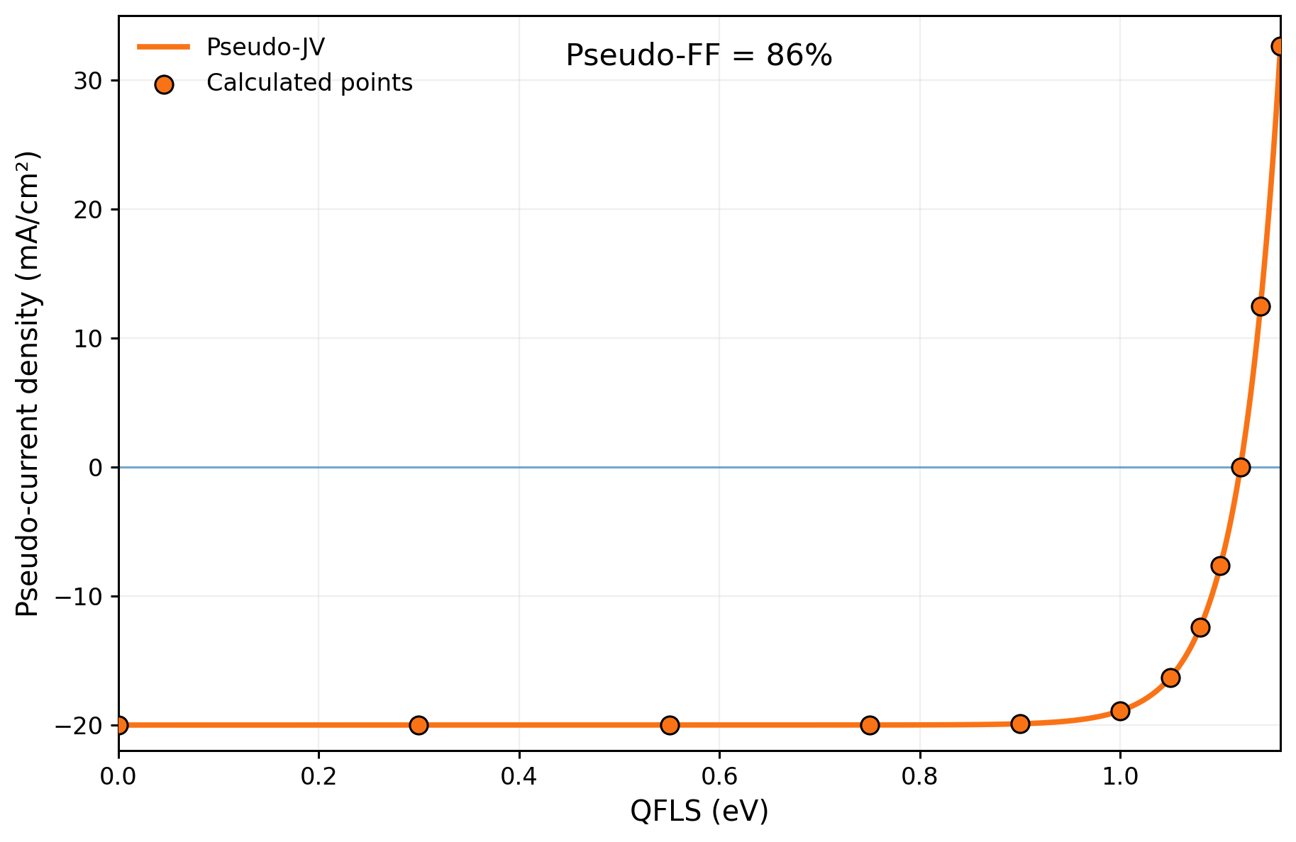
Intensity-dependent QFLS measurements contain more information than the ideality factor alone. By combining the measured QFLS with the corresponding excitation level, an implied current-voltage characteristic, commonly referred to as a pseudo-JV curve, can be reconstructed.
At each excitation intensity, the semiconductor reaches a steady-state carrier population characterized by a certain QFLS. Under open-circuit conditions, no net current is extracted, so photogeneration is balanced by recombination:
The QFLS defines the corresponding implied voltage:
At the same time, the calibrated excitation level determines the equivalent generation current density JG=qGd, where G is the generation rate per unit volume and d is the relevant absorber thickness. Under open-circuit conditions, this generation current is balanced by the recombination current:
An excitation-intensity sweep therefore provides a series of points relating recombination current density to implied voltage:
For the sign convention used in LuQY-Control, the illuminated pseudo-current density is written as
where JG,ref is the equivalent generation current density at the selected reference illumination.
At low QFLS, the recombination current is small and the pseudo-current approaches−JG,ref. As QFLS increases, recombination increases until
at which point
This point corresponds to the implied open-circuit condition.
The resulting curve resembles a conventional electrical JV characteristic and can be used to determine quantities such as the pseudo open-circuit voltage, the pseudo maximum-power point, and the pseudo fill factor (pFF).
What does the pseudo-JV tell us?
Unlike a conventional electrical JV measurement, the pseudo-JV curve is reconstructed from intensity-dependent luminescence measurements. During the QFLS measurement, current does not need to be extracted through the external device contacts.
The pseudo-JV therefore provides access to the recombination-limited performance potential of the measured material or device stack. Losses associated with the external electrical path, such as series resistance and charge-extraction limitations, are not included in the same way as in a conventional electrical JV measurement.
Comparing pseudo-JV and electrical JV characteristics can therefore help distinguish recombination losses from additional transport, contact, and resistive losses.
The pseudo fill factor (pFF) is particularly useful for this comparison. It describes the fill factor derived from the reconstructed recombination characteristic without the additional limitations of the external electrical path.
JV Metrics, Bandgap and EQE
From PL to the real device
For a photovoltaic device, the short-circuit current density, JSC, is the current density delivered when the device is operated at zero applied voltage and 1-sun illumination conditions. The open-circuit voltage, VOC, is the voltage at which no net current flows; it is closely related the separation of the electron and hole Fermi levels at the contacts. Together with the fill factor, these parameters determine the power conversion efficiency.
Absolute PL does not directly measure changes in JSC. Instead, it provides complementary information about the optoelectronic quality of the absorber and the device stack. It can help answer questions with indirect implications for photovoltaic parameters, such as:
‣ Are non-radiative losses limiting the achievable voltage of the device?
‣ Does the sample/material processing induce non-radiative decay channels that would impede the end device performance?
‣ Does a transport layer passivate the absorber or introduce interfacial losses?
‣ Are losses located in the bulk or at an interface?
‣ Does the luminescence track with device photocurrent as a function of applied bias?
‣ Are there spatial regions likely limiting device performance?
PL intensity alone therefore should not be treated as a direct prediction of JSC or efficiency. A strong PL signal may indicate low non-radiative recombination, but device performance also depends on absorption, charge extraction, transport resistance, contacts and parasitic losses.
With the integrated SMU in our LuQY Pro systems, the absolute PL of a complete device (and the PLQY) can also be compared at open circuit and at short circuit, revealing insights about bias-dependent carrier collection efficiency.
Efficient charge extraction strongly reduces the PL at short circuit, so this comparison gives a qualitative indication of how well photogenerated carriers are collected, which is directly relevant to JSC. By measuring around the maximum power point, the same is deduced for device operating conditions related to the FF.
Excitation intensity and sample bandgap
The bandgap sets the limits
A semiconductor's bandgap (Eg) decides which part of the solar spectrum it can absorb. In the ideal case within the detailed balance (DB) framework, every photon above Eg is absorbed and collected as one electron, and every photon below it is lost. This case gives the thermodynamic short-circuit current density, JSC,DB :
ΦAM1.5G is the photon flux of the standard solar spectrum at air mass 1.5. A smaller bandgap absorbs more photons and gives a higher JSC,DB. For example, JSC,DB is about 44 mA/cm² at 1.12 eV (silicon) and about 26-33 mA/cm² at 1.6-1.4 eV (a typical perovskite).
EQEPV: what a real device collects
Real devices fall short of this limit because of reflection, parasitic absorption and smeared absorption edge, and incomplete carrier collection. The external quantum efficiency, EQEPV(E), is the fraction of incident photons at each energy that come out as collected electrons. The real JSC is the EQEPV weighted by the solar spectrum:
Why excitation intensity matters for PLQY analysis
To estimate the "1-sun-equivalent" optical excitation flux for PL measurements, the bandgap and thermodynamic JSC are used. This importantly allows the QFLS and voltage loss calculated later to be relevant to understanding the end device, as mentioned earlier.
To approximate the sample bandgap in sharp-absorption edged materials like perovskites, the PL spectral peak position is a convenient, widely used approach. While the EQEPV inflection point (absorption edge) is a common way to determine the bandgap, both methods typically agree within a few tens of meV. Such a difference reflects in 2-3% changes in JSC,DB, and are therefore considered negligible. Where EQEPV or absorptance data are available, the inflection point is used as a more rigorous definition for detailed-balance analysis (as is the case with the LuQY systems, see below).
Note that photon reabsorption, tail states, or halide segregation can shift the PL peak to lower energies.
Estimating 1-sun intensity in LuQY systems
The software built in to the LuQY measurement systems, like the LuQY Pro and LuQY Scanner, estimates the 1-sun equivalent excitation flux with the bandgap from either PL or from the EQE.
In case of a new material where the EQE or device JSC,DB is not known, the PL peak approximates Eg, from which the software calculates JSC,DB and assumes a practical working device reaches 85% of it. That is, the excitation intensity is set so that the carriers produced would generate a current of Jsc ≈ 0.85 JSC,DB. At such carrier density, an assumed EQEPV of 90% covers reflection and other optical losses in the sample. If these values are already known to user, the user may enter the device's actual Jsc, or upload the EQEPV file, for a rigorous setting of the 1-sun-equivalent intensity. In the case of an uploaded EQEPV file, the software uses the EQEPV inflection point to obtain the sample bandgap.
Electroluminescence: same relation, driven by voltage
Reciprocity also works in reverse for finished devices. If a solar cell is run as an LED under forward bias, its absolute EL spectrum is tied directly to its photovoltaic EQE (Rau):
Measuring absolute EL is therefore an independent route to the device's EQEPV, especially near and below the band edge:
‣ Band-edge and sub-gap EQEPV: EL is strongest exactly where conventional EQEPV measurements run out of signal. Dividing the EL spectrum by ΦBB reconstructs the EQE edge, Urbach tail and sub-gap states over several orders of magnitude. Note that for measurement of EL without a high-sensitivity lock-in amplifier, a considered extrapolation of the EL signal could resolve EQEPV well beyond the bandgap region.
‣ Radiative limit without a separate EQE setup. The same spectrum gives J0,rad and therefore Voc,rad.
‣ Non-radiative voltage loss from the LED efficiency. The external EL quantum efficiency (ELQY) gives the device's non-radiative loss directly: ΔVoc,nr = −(kT/q) ln(ELQY). This mirrors the PLQY relation above, but for the complete device including its contacts.
Absolute PL Mapping
Quantifying PL images
A single-point PL measurement only probes the area under the excitation spot. PL mapping scans the excitation across the sample and records the luminescence at each position, showing how the emission varies across the surface. Spatial uniformity matters most when a small measurement spot is used to assess a large-area film or device.
A strong emission at one location may not be representative of the whole sample spectral properties.
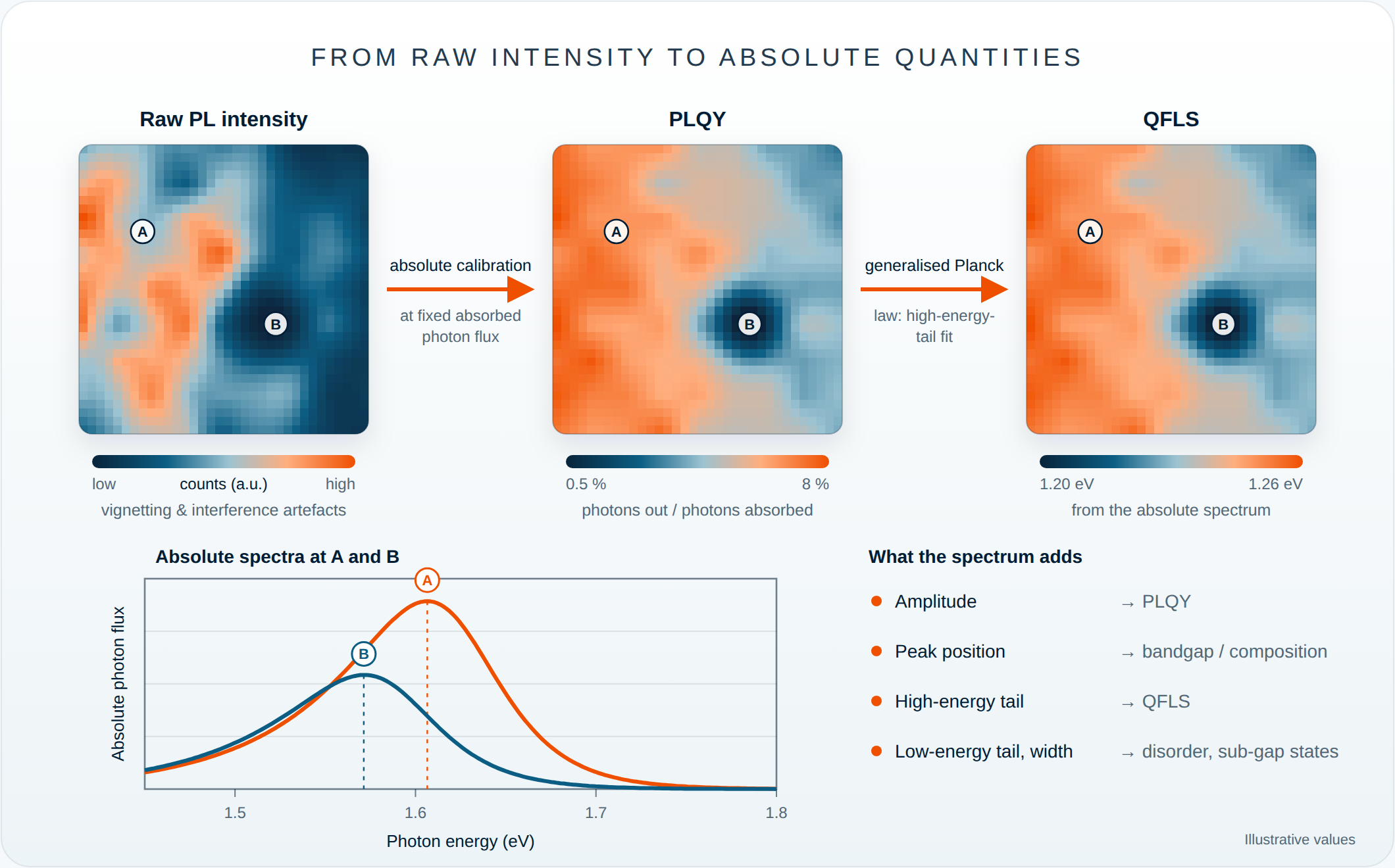
Variations in a PL intensity map can have many causes. Some originate in the sample: local differences in non-radiative recombination (e.g. defect clusters or grain boundaries), bandgap or compositional variation, phase segregation, or thickness variation. Others originate in the measurement: non-uniform excitation intensity or focus, sample tilt, substrate reflectance, interference, and differences in outcoupling or collection geometry. Raw PL intensity maps are therefore a useful qualitative indicator of uniformity, but on their own they do not give a quantitative measure of material quality.
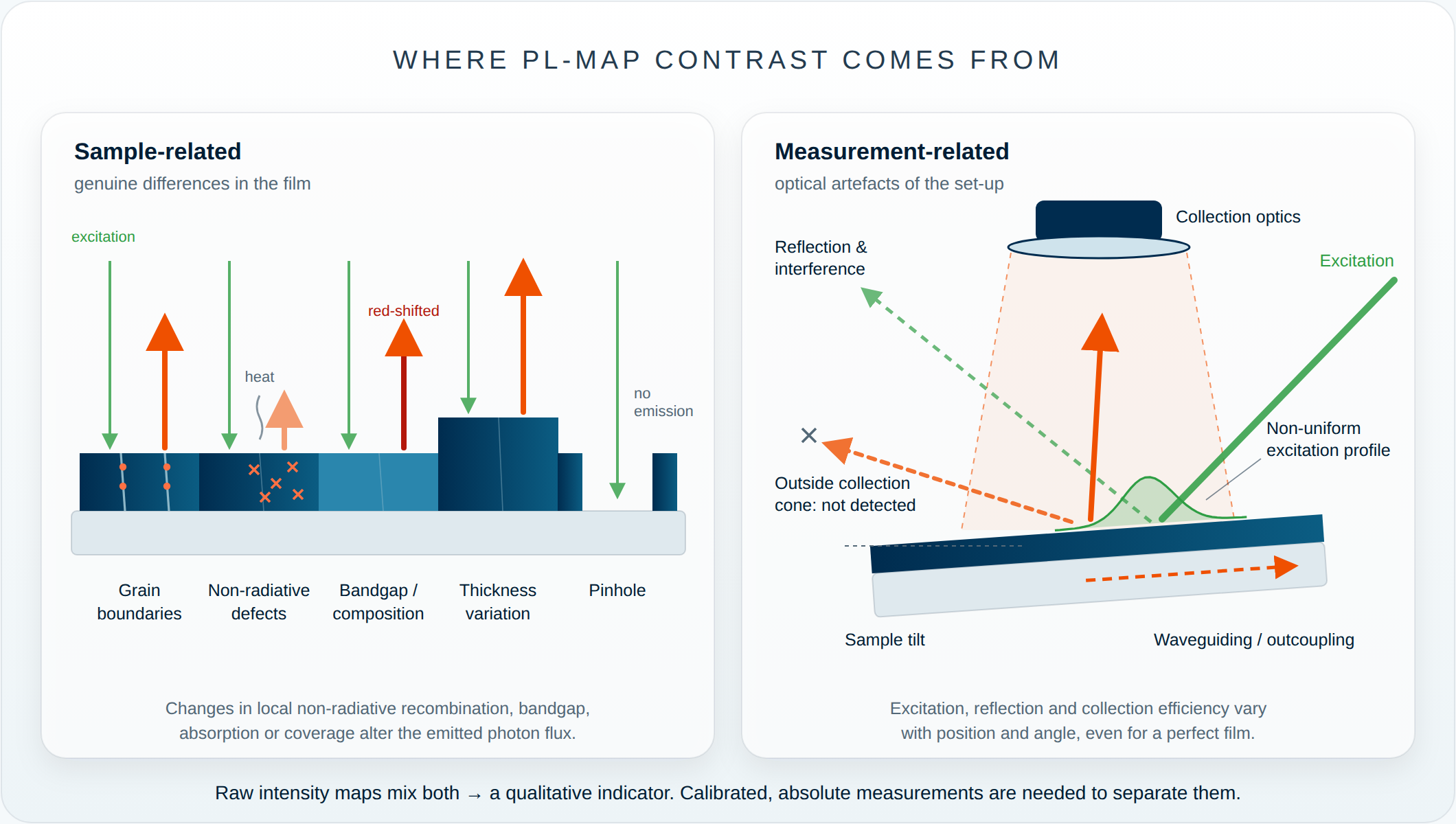
Mapping absolute PL, followed by local analysis of PLQY or QFLS, provides much more information than raw intensity alone. QFLS can be extracted from the absolute PL spectrum, provided the spectral calibration is accurate. Because PLQY and QFLS depend on excitation intensity, measurements should be compared at the same absorbed photon flux, typically 1-sun equivalent. Calibrated measurements under these conditions help separate real variations in film quality from optical artefacts, and are therefore more powerful than standard PL imaging. For instance, the LuQY Scanner resolves the absolute spectral photon flux and emission yield at each point, which helps identify the physical origins of variations in the PL map.
Sample uniformity and stack quality
Quantitative emission characteristics of the sample obtained from mapping absolute PL can then be linked to material quality, processing conditions or growth control, among other factors.
Spatially resolved PL can be used to investigate:
‣ Film uniformity
‣ Local defects
‣ Thickness, composition or bandgap gradients
‣ Pinholes and incomplete coverage
‣ Grain-to-grain variation (where the spatial resolution is finer than the grain size)
‣ Processing non-uniformity
‣ Localised or edge-initiated degradation
‣ Quality across large-area samples
Comparing the absolute emission of a bare absorber with that of the same absorber after adding transport layers or contacts can help identify losses at interfaces. Under steady-state, open-circuit conditions, a drop in PLQY or QFLS after adding a charge-transport layer usually points to additional non-radiative recombination at the interface or to unfavourable energy-level alignment. Changes in optical outcoupling or parasitic absorption in the added layer can also contribute. Time-resolved PL can help distinguish charge extraction from interfacial recombination.
Spectrally resolved absolute PL mapping therefore gives detailed insight into how the physical properties of a sample vary across its area, particularly when combined with:
‣ PLQY
‣ QFLS, or equivalently the implied open-circuit voltage (iVOC = QFLS/q)
‣ Excitation-intensity dependence, which gives the ideality factor, pseudo-JV curves and the dominant recombination regime)
‣ Measurements of systematically varied layer stacks
Comparing the QFLS of the absorber, partial stacks and the complete device can show whether performance is limited mainly by bulk material quality, surface passivation, transport layers, interfaces or contacts. Comparing the QFLS of the full device with its measured VOC then reveals any further losses from the contacts or from energy-level alignment.
Questions & Answers
What is photoluminescence quantum yield (PLQY)?
PLQY is the fraction of absorbed photons that a material re-emits as light: emitted photons by absorbed photons. It quantifies how efficiently absorbed optical energy is converted into luminescence and is sensitive to non-radiative recombination losses.
Read the full theory Absolute Luminescence and Quantum YieldHow is PLQY measured with an integrating sphere?
An integrating sphere is a hollow sphere with a highly reflective inner coating that collects emitted light over a wide range of angles. It enables the emitted and absorbed photon fluxes to be quantified when precisely calibrated. In other words, accurate PLQY measurements require calibrated spectral response and careful treatment of excitation light, sample geometry and optical losses.
Read the full theory Absolute Luminescence and Quantum YieldWhat is the difference between absolute and relative photoluminescence?
Relative PL describes spectral shape or intensity in arbitrary units, while absolute PL determines the emitted photon flux on a calibrated scale. Absolute measurements make it possible to calculate quantities such as PLQY and QFLS.
Read the full theory Absolute Luminescence and Quantum YieldWhat is the difference between PLQY and ELQY?
PLQY describes luminescence efficiency under optical excitation, whereas ELQY describes the emitted photon yield under electrical injection. Both quantify radiative emission efficiency but use different excitation mechanisms.
Read the full theory Absolute Luminescence and Quantum YieldHow are PLQY and ELQY of a sample related?
If every injected charge reaches the active layer and recombines there, ELQY equals PLQY at the same carrier density. In real devices, ELQY ≈ PLQY × the fraction of injected charge that recombines in the active layer, describing the contribution on non-radiative to loss in charges, for example at the contacts or transport layers. Both parameters relate to non-radiative losses logarithmically: about 60 mV rise in voltage losses for every tenfold drop in quantum yield below 100%.
Read the full theory Quasi-Fermi-Level SplittingWhat is quasi-Fermi-level splitting (QFLS)?
QFLS is the energy that separates steady-state electron and hole populations in a semiconductor in non-equilibrium conditions. It provides a measure of the internal voltage potential of an excited semiconductor absorber.
Read the full theory Quasi-Fermi-Level SplittingWhat is the difference between QFLS, iVoc and Voc?
QFLS is the energetic analogue to the implied open-circuit voltage, iVOC. Their relation is given by iVOC = QFLS/q. The QFLS and iVOC can be indirectly measured for a standalone film or a sample stack without contacts, via the absolute PL spectrum of that stack. The terminal VOC is measured electrically across the full device stack. If the device is additionally be affected by contact-, transport- or interface losses then the VOC drops below the iVOC.
Read the full theory Quasi-Fermi-Level SplittingHow is QFLS determined from absolute photoluminescence?
A calibrated absolute PL spectrum contains information about the carrier populations in the absorber. By analysing the emission spectrum, including its high-energy tail, QFLS can be extracted under defined excitation conditions.
Read the full theory Quasi-Fermi-Level SplittingWhat is the relationship between PLQY and QFLS?
Both quantities are influenced by radiative and non-radiative recombination. Under comparable measurement conditions, reduced non-radiative losses generally lead to higher PLQY and a larger QFLS.
Read the full theory Quasi-Fermi-Level SplittingHow are PLQY and non-radiative voltage loss related?
PLQY provides a direct measure of the fraction of recombination that produces luminescence. A lower external luminescence efficiency corresponds to a larger non-radiative voltage loss relative to the radiative limit.
Read the full theory Quasi-Fermi-Level SplittingWhat is the ideality factor and how can it be determined from photoluminescence?
The ideality factor describes how the recombination behaviour, and therefore QFLS, changes with carrier density or excitation intensity. It can be determined from the dependence of QFLS on the logarithm of the generation rate, i.e., the excitation intensity.
Read the full theory Ideality FactorHow does excitation intensity affect PLQY and QFLS?
Changing excitation intensity changes the carrier density and therefore the balance between different recombination pathways. For example, every tenfold increase in intensity raises the QFLS by 60 mV x nid. Intensity-dependent measurements can reveal trap filling, bimolecular recombination and higher-order loss processes.
Read the full theory Ideality FactorHow is 1-sun-equivalent excitation determined in a PL measurement?
A 1-sun-equivalent condition is defined by matching the photogenerated carrier flux to that expected under the AM1.5G solar spectrum. The conversion depends on the absorber bandgap, spectral response and excitation wavelength.
Read the full theory JV Metrics, Bandgap and EQEWhat is the bandgap of a semiconductor and how can it be determined?
The bandgap is the minimum energy needed to excite an electron from the valence to the conduction bands. It determines which photons a material can absorb, and is related to the upper limit of the voltage achievable across the material. It is determined from the inflection point of the photovoltaic external quantum efficiency spectrum, or approximated by the peak PL emission energy for materials with sharper absorption edges.
Read the full theory JV Metrics, Bandgap and EQEWhat is external quantum efficiency (EQE)?
EQE describes the fraction of incident photons at a given wavelength that contribute to collected electrical charge in a photovoltaic device. It connects the spectral response of the device to its photocurrent.
Read the full theory JV Metrics, Bandgap and EQEHow is Jsc calculated from EQE?
The short-circuit current density is obtained by weighting the device EQE with the AM1.5G solar photon flux and integrating over photon energy or wavelength. This gives the expected photocurrent under standard solar illumination.
Read the full theory JV Metrics, Bandgap and EQEWhat is a pseudo-JV curve?
A pseudo-JV curve reconstructs the internal recombination-limited current–voltage behaviour from intensity-dependent luminescence measurements. It can be used to estimate device performance without requiring a conventional electrical JV sweep.
Read the full theory Pseudo-JV CurvesWhat information can absolute PL mapping provide?
Absolute PL mapping spatially resolves quantities such as emission intensity, PLQY, QFLS or implied voltage across a sample. It can reveal local non-uniformities, defects and spatial variations in material or device quality.
Read the full theory Absolute PL MappingWhy is calibration important in absolute photoluminescence measurements?
Absolute measurements require the detected signal to be converted into a physically meaningful photon flux, since the spectrometer and integrating sphere do not share responsivity at all wavelengths. Spectral sensitivity, optical losses, excitation power and collection geometry therefore need to be characterised and calibrated.
Read the full theory Absolute Luminescence and Quantum YieldReferences
- Unold, T.; Gütay, L. Photoluminescence Analysis of Thin-Film Solar Cells. In Advanced Characterization Techniques for Thin Film Solar Cells; Wiley-VCH Verlag GmbH & Co. KGaA, 2011; pp 151–175.DOI ↗
- Kirchartz, T.; Márquez, J. A.; Stolterfoht, M.; Unold, T. Photoluminescence-Based Characterization of Halide Perovskites for Photovoltaics. Adv. Energy Mater. 2020, 1904134.DOI ↗
- Swartz, C.; Paul, S.; Mansfield, L.; Holtz, M. Absolute photoluminescence intensity in thin film solar cells. Journal of Applied Physics 125, 053103, 2019.DOI ↗
- Rau, U. Reciprocity relation between photovoltaic quantum efficiency and electroluminescent emission of solar cells; Phys. Rev. B 76, 085303, 2007.DOI ↗