
Research questions to measurement workflows

Applications

Explore how absolute PL and TRPL measurements answer concrete research questions in solar cells, light-emitting devices, materials development and sample processing. Each field connects the measurement approach with the QYB system suitable for the workflow.

Click on scientific terms such as QFLS and PLQY or on instrument names like LuQY Pro to learn more.

Applications · Photovoltaics

Solar cells

Use absolute luminescence to locate voltage, recombination, transport and uniformity losses from absorber films to complete solar cells and modules.
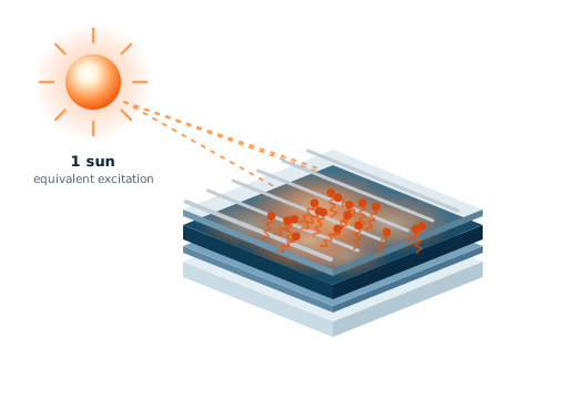
Layer-by-layer loss analysis

Question

How much of the difference between sample voltage and its radiative limit is caused by the bulk absorber, by each interface and by transport to the contacts?

Measurement

PLQY and QFLS are measured at the 1-sun-equivalent generation rate on a sequence of samples: the neat absorber, the absorber with each transport layer (half-stacks), the full stack and the finished cell. Excitation-intensity sweeps on each sample give pseudo-JV curves. The SMU records the electrical J–V curve of the finished cell. ELQY measured with 1-sun-equivalent injected current on the full stack independently cross-checks losses.

Instrument: LuQY Pro for single sample, LuQY Scanner for all samples in the sequence (+mapping, see here)

What you learn · each stack step isolates one loss

  • Neat absorber: non-radiative loss in the bulk and at free surfaces, ΔVnr = −(kBT/q) ln(PLQY), relative to the radiative limit.
  • Half-stacks: additional recombination introduced by each interface, such as SAM layers, transport layers or buffer layers/interlayers for tandem cells. The interface that lowers the QFLS most is the first target for passivation [3].
  • Finished cell: the difference between QFLS and qVOC, and the difference between the pseudo fill factor and measured fill factor. The latter separates recombination-limited fill factor from transport and series-resistance losses.
  • Implied efficiency of the end device: Intensity sweeps on the neat absorber and subsequent stacks also give the implied efficiency: the efficiency a stack or device could reach if carrier collection introduced no further losses [4]. It is defined using iVOC (or pseudo-VOC), the pseudo-FF and the short-circuit photocurrent. The maximum power output is marked by the pseudo maximum-power point. Plotting the pseudo-JV parameters alongside QFLS for each stack gives predictive insight into sequential losses before the device is fully built.
  • PLQY of 10-100% → Interpreted as nearly all radiative recombination. Indicates excellent material quality (like GaAs).
  • PLQY of 0.1-10% → Increased fraction of non-radiative losses; still allowing for highly efficient solar cells (e.g. world record cells in perovskites).
  • PLQY of 0.01 – 0.1% → Significant non-radiative losses; material still usable but improvements recommended.
  • PLQY< 0.01% → Dominant non-radiative recombination; poor optoelectronic quality.
Considerations for interpretation

The QFLS losses of the individual layers do not simply add up. The QFLS is the logarithm of the recombination current, and is therefore dominated by the strongest recombination channel across the stack. [3] Samples should be compared on the same substrate type and at the same absorbed photon flux.
QFLS is generally an accurate predictor of the external device Voc, but can deviate from this value under strong mismatch of transport layer work functions, low mobility of absorber layers or interlayers, mobile ion & field-screening effects, etc. [2]

For finished devices, electroluminescence provides an independent cross-check. If the cell is driven with an injected current density equal to its JSC, the optoelectronic reciprocity relation [5] gives Eq. (A1) below. Note that this assumes reciprocity which holds when charge collection does not depend strongly on voltage. This should be checked for each device type.

ΔVOC,nr = − kBT q ln(ELQY)
(A1)

Spatial uniformity and upscaling

Question

Does the whole area of a large film or module reach the quality of the best spot, and where are the losses?

Measurement

Absolute PL mapping and PL imaging over areas up to 210 × 210 mm, either as one large sample or several smaller samples in one run.

Instruments: LuQY Scanner for large areas and sample throughput; LuQY Pro for single-sample mapping.

What you learn

  • Coating gradients, i.e. inconsistencies in film coating
  • Local defects and potential shunt channels
  • Edge effects, poor passivation and potential source points of sample degradation
  • Damage during post-processing, eg. dewetting or damage near module scribe lines
  • Intensity sweeps map the pseudo-FF across the film, showing where recombination limits the achievable fill factor before a device is built.
  • With upscaling, several samples are measured in one go, enabling statistics and correlation across large data sets.
Considerations for interpretation

The intensity gradients from the PL image cannot be used as a heuristic to access spatial variation in QLFS. More accurately, it is extracted from the local PLQY, which can be obtained only with local spectral analysis, as performed by the LuQY systems. This resolves potential spectral shifts across different measurement points. In finished devices with conductive electrodes, lateral currents redistribute voltage, so a local defect such as a shunt can appear as an extended dark region.

Stability: which loss appears first?

Question

When a device or film degrades, does it lose material quality, change composition, or do the interlayers and contacts deteriorate?

Measurement

Absolute PL spectra are recorded as a time series under continuous illumination at a fixed intensity. For complete devices, the SMU can simultaneously hold open circuit, a fixed voltage near the maximum power point, or a constant injected current.

Instruments: LuQY Pro; LuQY Lifetime for TRPL before and after.

What you learn → signatures differ by mechanism

  • PLQY and QFLS fall together: non-radiative recombination is increasing, for example through defect formation or interface degradation.
  • Red-shifted emission or an emerging low-energy band: this can indicate light-induced halide segregation in mixed-halide perovskites [6]. Recovery in the dark indicates a reversible fundamental process.
  • VOC falls while QFLS stays constant: the losses are located at the contacts rather than in the absorber.

    Note light soaking effects on PLQY: Under extended illumination, PL intensity can increase (photobrightening) or decrease (photodarkening), often depending on the atmosphere.

Voltage-resolved absolute PL

Question

Where between open-circuit and short-circuit does a device lose internal voltage, and how efficiently are photogenerated carriers extracted?

Measurement

The complete cell is illuminated at the 1-sun-equivalent generation rate while the integrated source-measure unit (SMU) sets the terminal voltage, stepping from VOC through the maximum power point to 0 V (short circuit). At each step the absolute PL spectrum is recorded and the QFLS is extracted.

Instrument: LuQY Pro.

What you learn

  • At open circuit, comparing QFLS with qVOC shows whether the full internal voltage reaches the terminals. A QFLS clearly above qVOC points to energetic misalignment of transport layers, non-ideal contacts or ionic field screening, among other causes [1, 2].
  • At operating voltages, the difference QFLS − qV is the part of the internal voltage that is lost on the way to the contacts. If this difference grows towards the maximum power point, the fill factor is limited by transport and extraction rather than by recombination alone.
  • Towards short circuit, efficient extraction lowers the steady-state carrier density in the absorber, so the PL is strongly quenched. A PL signal that remains high at short circuit indicates that a substantial fraction of carriers recombines before it is collected, which is directly relevant to JSC.
Considerations for interpretation

When the device delivers current, meaning that the SMU sinks rather than injects current, the extraction of current needs to be considered as a competition to emissive recombination pathways. In this case, the generalized LuQY of Eq. (5) on the absolute PL theory page is dealt with careful consideration.

Applications · LEDs

Light-emitting devices

Combine calibrated EL and PL measurements to separate emitter quality, charge balance, exciton utilization, outcoupling and electrical efficiency.

LED efficiency loss analysis

Question

Is an LED limited by its emitter material, by charge balance, or by light outcoupling?

Measurement

The SMU sweeps the drive current while the absolute EL spectrum and ELQY are recorded. The PLQY of the emissive layer is measured separately, both on its own and in half-stacks.

Instrument: LuQY Pro.

What you learn

  • Outcoupling efficiency: Because the integrating sphere collects light emitted in all directions, the ELQY can be equated with the EQEEL and factorized as the product of γ, ηEUE, ηrad, and ηout. Here γ is the charge-balance factor: the fraction of injected electrons that successfully form an electron–hole pair or exciton in the emitter. It is unity in an ideal stack and is affected mainly by transport and injection layers. ηEUE, the exciton-utilization efficiency, describes how many formed excitons are emissive, including how many triplet states contribute to emission. ηout is the outcoupling efficiency. Since the PLQY gives ηrad, the ratio of ELQY to PLQY indicates how much is lost to charge balance and outcoupling when ηEUE is known.
  • ELQY versus current density, including efficiency roll-off at high current
  • Spectral properties: Peak position, line width and CIE colour coordinates from the absolute spectrum, and spectral stability under bias
  • Wall-plug (power conversion) efficiency, from the calibrated optical output power divided by the electrical power I·V from the SMU.

    Because every LED is also a photovoltaic diode, ELQY measured at an injection current equal to JSC quantifies the non-radiative voltage loss of a solar cell, as in Eq. (A1) in the solar-cell applications section above. LED and solar-cell research therefore share a common measurement.
Considerations for interpretation

Film PLQY is itself an external yield and depends on carrier density, so it should be compared with the device at a similar carrier density as the ELQY. Matching emitted photon flux or QFLS is a practical way to do this. The sphere also collects light escaping through substrate edges, which forward-viewing setups miss, so sample geometry should be comparable, especially when comparing literature values.

Instrument range

The integrated SMU in LuQY Pro can provide up to 150 mA and ±10 V bias. For greater biasing ranges, an upgraded SMU is possible, or an electrical feedthrough can interface the system with an external SMU.

Applications · Materials

Materials science and further fields

Connect absolute quantum yield with time-resolved photoluminescence to understand recombination rates, treatments, carrier-density regimes and photoelectrochemical loss budgets.

Process control & recombination rates

Question

Does a treatment make a material brighter by removing non-radiative channels or by speeding up radiative emission?

Measurement

PLQY and the TRPL decay are measured on the same sample, at the same excitation wavelength and comparable excitation density.

Instruments: LuQY Pro and LuQY Lifetime.

What you learn

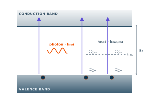
  • For an emitter with first-order kinetics, such as molecules, quantum dots or a doped semiconductor in low injection, PLQY = krad/(krad + knon,rad) and the PL lifetime is τ = 1/(krad + knon,rad). The two rates follow Eq. (A2) below.
  • Note: A shorter lifetime alone is ambiguous. Combined with PLQY it shows whether ligand exchange, shell growth, doping or a new passivation layer reduced knon,rad or increased krad. TRPL alone cannot make this distinction, and PLQY alone cannot either.
krad= PLQYτ , knon,rad= 1−PLQYτ
(A2)
Considerations for interpretation

Eq. (A2) is exact only for a single-exponential decay. For multi-exponential decays, a properly weighted average lifetime gives an effective rate and this should be stated. Measured PLQY is external, so photon recycling and outcoupling make krad an apparent rate. In thin films of halide perovskites at solar-relevant carrier densities, radiative recombination is bimolecular and both rates depend on carrier density. Delayed emission, for example from TADF emitters, contributes to PLQY and must fall within the TRPL time window to be captured by τ.

Perovskite decays

Lead-halide perovskite PL decays measured at high fluence require careful fitting because PL intensity can follow a power-law dependence with time. Simple exponential fits can misinterpret the data and hide measurement-condition dependence [7].

Dominant recombination regimes

Question

At the carrier densities where a material operates, which recombination process dominates, and how does a treatment change it?

Measurement

PLQY is measured over several decades of excitation intensity, with the 1-sun-equivalent point marked, and complemented by a TRPL series at different excitation fluences.

Instruments: LuQY Pro and LuQY Lifetime.

What you learn → Intensity dependence

  • In the simplified ABC description from the TRPL theory page, with n ≈ p ≈ Δn, the internal radiative efficiency is:
    PLQYint = BΔn / (A + BΔn + CΔn2)

    The same sweep yields the ideality factor. If emitted flux scales as exp(QFLS/kBT), the slope of PLQY versus generation rate G is linked to nid by:
    PLQY ∝ G(nid − 1)

    Thus nid = 2 corresponds to PLQY rising linearly with intensity, while nid = 1 corresponds to constant PLQY. The TRPL fluence series provides an independent measurement: trap filling appears as a slower early decay at higher fluence, while higher-order recombination appears as a faster one.
  • PLQY rising in proportion to intensity: trap-assisted (first-order) recombination dominates, and increasing intensity fills or outcompetes traps.
  • PLQY approximately constant: radiative recombination dominates, or the material is doped (see limits below).
  • PLQY falling at high intensity: Auger-type or other higher-order losses set in.
Considerations for interpretation

In a doped semiconductor under low injection, radiative recombination is also first-order (rate ∝ NdopΔn), so constant PLQY does not by itself prove radiative dominance. The doping level must be known. Sample heating and photobrightening at high intensity can distort the sweep; measuring with increasing and then decreasing intensity is a useful check. Generation rates should be stated as absorbed photon flux.

Photoelectrochemistry and photocatalysis

Measurement insight

In a photoelectrode for solar fuels, the QFLS of the absorber sets the upper limit of the photovoltage available to drive the reaction.

Comparing the QFLS of the bare absorber with that of the absorber carrying protection layers and co-catalysts shows how much voltage each layer costs. This is the same loss-budget logic used for solar-cell stacks. Absolute PLQY of photocatalyst films likewise quantifies non-radiative losses before electrochemical testing.

Applications · Integrated Platforms

Integrated Platforms

Scale your workflow by combining LuQY measurement systems with material acceleration platforms and more. For fully automated & high-throughput optoelectronic characterization.

Automated high-throughput workflows

Question

How to combine high-throughput sample processing with feedback from absolute optoelectronic measurements?

Integrated solution

Automated characterization platform by SCIPRIOS × QYB

SCIPRIOS provides the robotic infrastructure for high-throughput sample fabrication and transfer to the optoelectronic module from QYB which runs quantitative optical and optoelectronic characterization. The hardware and software of both modular units communication with one another for a streamlined workflow without repeated manual handling.

Scientific basis

References

  1. [1]P. Caprioglio et al., On the relation between the open-circuit voltage and quasi-Fermi level splitting in efficient perovskite solar cells, Advanced Energy Materials 9, 1901631 (2019).
  2. [2]R. Warby et al., Mismatch of quasi-Fermi level splitting and VOC in perovskite solar cells, Advanced Energy Materials 13, 2303135 (2023).
  3. [3]M. Stolterfoht et al., Visualization and suppression of interfacial recombination for high-efficiency large-area pin perovskite solar cells, Nature Energy 3, 847–854 (2018).
  4. [4]M. Stolterfoht et al., How to quantify the efficiency potential of neat perovskite films: perovskite semiconductors with an implied efficiency exceeding 28%, Advanced Materials 32, 2000080 (2020).
  5. [5]U. Rau, Reciprocity relation between photovoltaic quantum efficiency and electroluminescent emission of solar cells, Physical Review B 76, 085303 (2007).
  6. [6]E. T. Hoke, M. D. McGehee et al., Reversible photo-induced trap formation in mixed-halide hybrid perovskites for photovoltaics, Chemical Science 6, 613–617 (2015).
  7. [7]Y. Yuan, T. Kirschartz et al., Understanding Power-Law Photoluminescence Decays and Bimolecular Recombination in Lead-Halide Perovskites, Advanced Energy materials, 15, 6, 2403279 (2025)
  8. [7]T. Kirchartz, scientific analysis of photoluminescence transients and recombination in photovoltaic materials, Advanced Energy Materials (2024).